The Data Menu

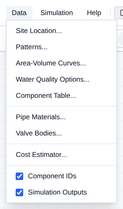
The Data menu holds project-wide libraries and settings: site climate, demand patterns, tank geometry, water quality, a spreadsheet of components, pipe materials, valve bodies, and the cost estimator. Define these once and reference them from individual components.

Here is a breakdown of every option in the Data menu:

• Site Location...: Latitude, longitude, and fetched climate used by solar/wind generators and regional cost defaults.
• Patterns...: Time-varying multipliers for demand, energy rates, and similar 24-hour or 12-month schedules.
• Area-Volume Curves...: Elevation–area–volume tables for non-cylindrical tanks.
• Water Quality Options...: Enable chemical, age, source-trace, or MSX analysis for the hydraulic run.
• Component Table...: Spreadsheet view of pipes, nodes, and other types, with CSV export.
• Pipe Materials...: Roughness C plus elastic properties used for friction and surge wave speed.
• Valve Bodies...: Fully-open minor-loss K values referenced by valves.
• Cost Estimator...: Bill of materials and unit prices, including power/fuel rates.
• Component IDs: Show or hide ID labels on the canvas.
• Simulation Outputs: Show or hide live result labels on the canvas.

Site Location

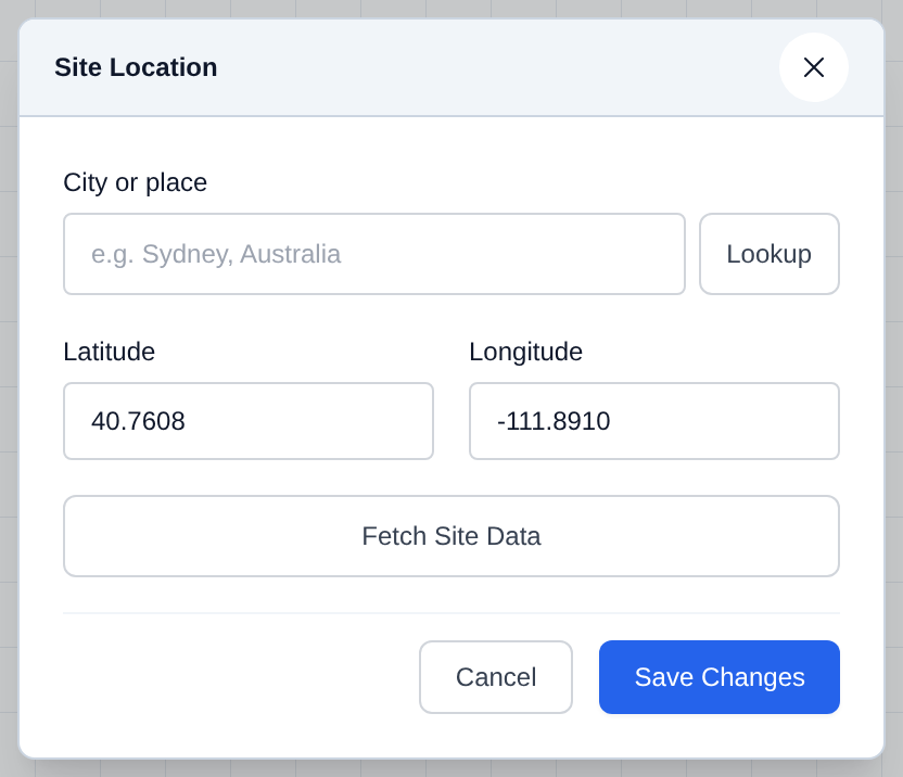
Open Data → Site Location... to place the project on the map. Solar and wind generators use the fetched climate (temperature, solar radiation, wind, sunrise/sunset). After a fetch you can also apply regional energy-rate, currency, and CapEx defaults used by the Cost Estimator.

For sources, forecast horizon, and fallbacks, see Appendix F: Site Weather Data.

1. Open Data and choose Site Location....
2. Type a city and click Lookup, or enter Latitude and Longitude directly.
3. Click Fetch Site Data.
4. Click Save Changes.

To refresh climate later without reopening this dialog, click the Weather HUD on the canvas and choose Fetch Weather Data. That writes the new forecast immediately and does not change regional cost defaults. See The Canvas.

Patterns

Open Data → Patterns... to build multipliers that scale a base value over time. Outflow nodes use them for demand; the Cost Estimator can use them for time-of-use energy prices.

1. Open Data and choose Patterns....
2. Click New Pattern.
3. Set Pattern Name and Pattern Type (Diurnal 24 hours, or Seasonal 12 months).
4. Edit multipliers in the table, or drag points on the chart (1.0 = the base value).
5. Click Save & Close. Then pick that pattern on the component that should use it.

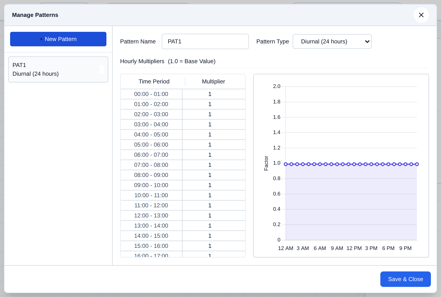
[!TIP] Dragging points on the chart is often faster than typing every multiplier.

Area-Volume Curves

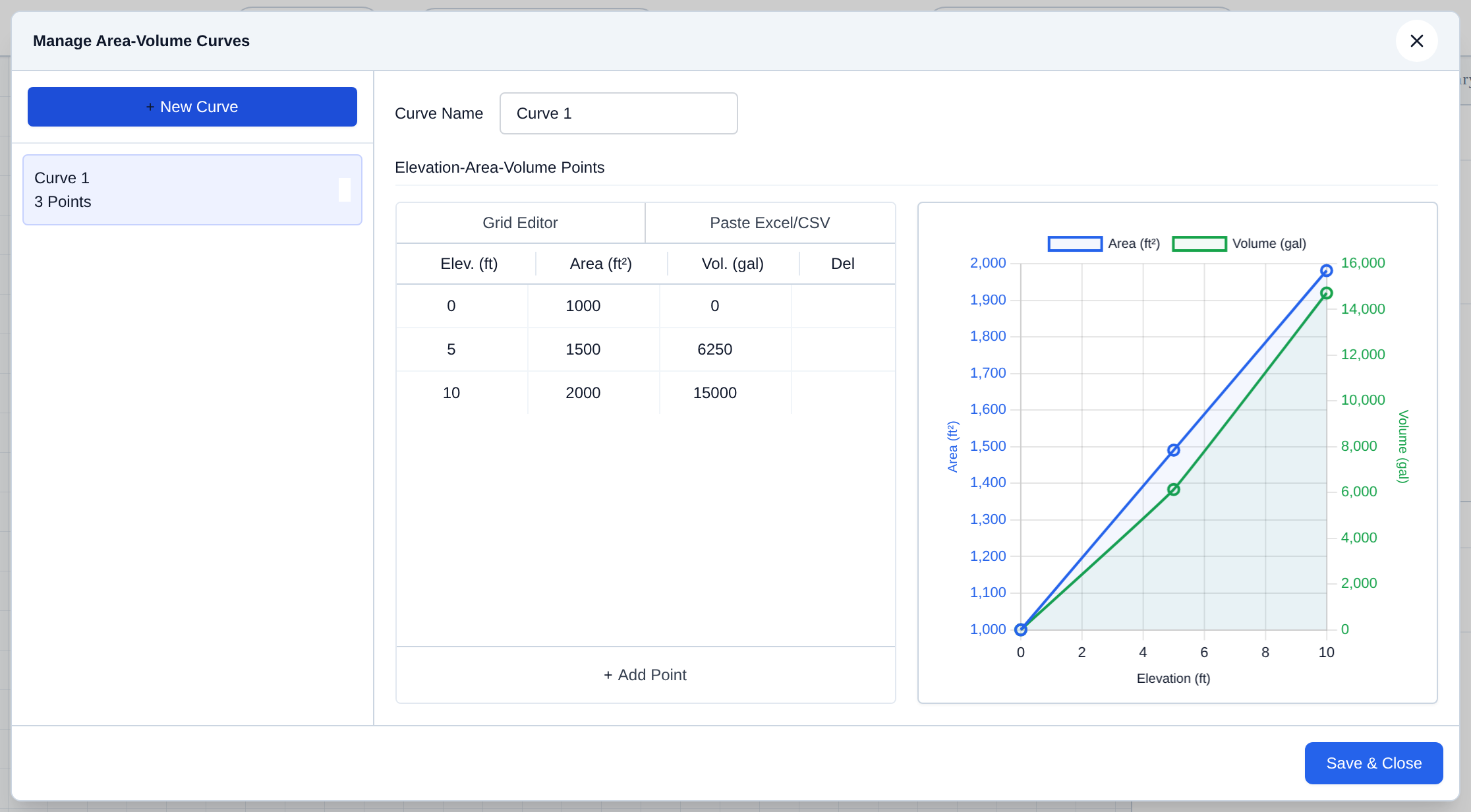
Open Data → Area-Volume Curves... when a tank is not a simple cylinder. Assign the curve on the tank so stored volume follows the elevation–area–volume table.

1. Open Data and choose Area-Volume Curves....
2. Click New Curve and name it.
3. Enter points in the Grid Editor, or use Paste Excel/CSV (Elevation, Area, Volume).
4. Click Save & Close. Then select the curve on the tank.

Water Quality Options

Open Data → Water Quality Options... to track a constituent, water age, a source trace, or an MSX multi-species model during the hydraulic run. Junction, tank, and source properties supply initial concentrations and source strengths after you enable this.

1. Open Data and choose Water Quality Options....
2. Check Enable Water Quality Analysis.
3. Choose Analysis Type: Chemical / Constituent, Water Age, Source Trace, or Multi-Species Extension (MSX).
4. Fill the fields for that type (chemical name and units, trace node, reaction coefficients, or MSX template).
5. Click Save Changes.

Component Table

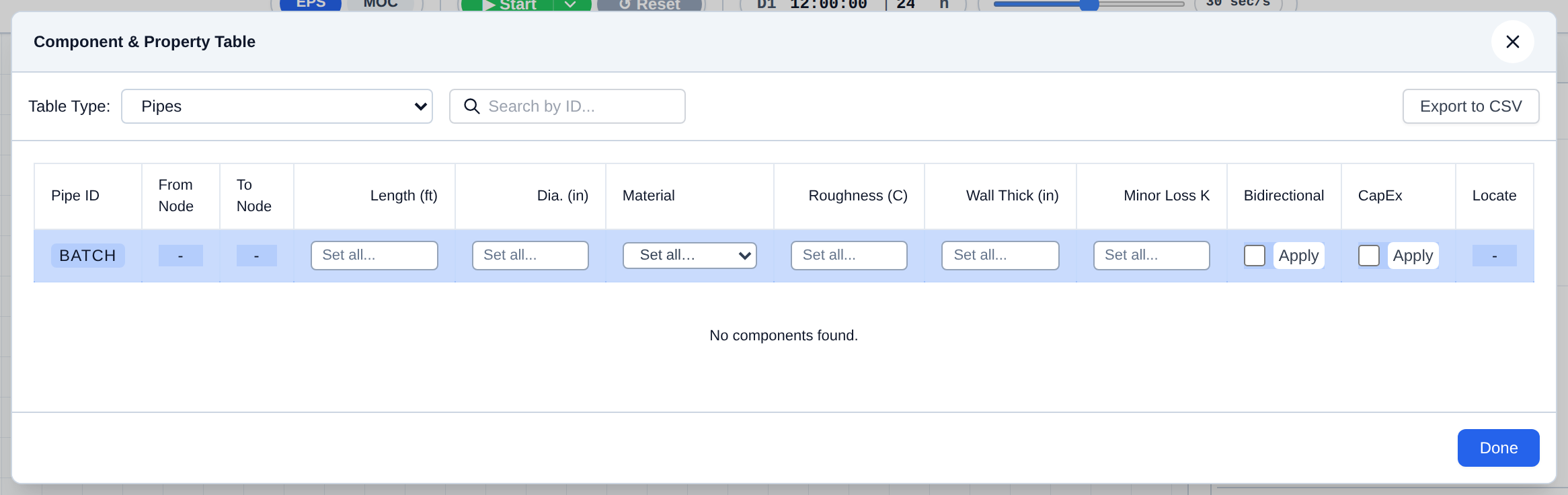
Open Data → Component Table... to review or batch-edit many components of one type without opening each properties dialog. Useful for diameters, roughness, elevations, and similar fields across a large network.

1. Open Data and choose Component Table....
2. Pick a Table Type (Pipes, Junctions, Storage, Pumps/Turbines, Valves, and so on).
3. Search by ID if needed. The blue header row can apply a value to every row.
4. Optionally Export to CSV.
5. Click Done.

Pipe Materials

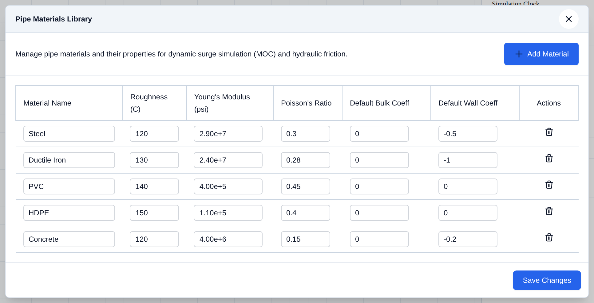
Open Data → Pipe Materials... to maintain the pipe materials library that pipes reference. Roughness (C) is used for friction in the hydraulic run. Young's Modulus and Poisson's Ratio are used for wave speed in a Method of Characteristics (MOC) surge run. Bulk and wall coefficients are defaults for water-quality reactions.

1. Open Data and choose Pipe Materials....
2. Edit a row or click Add Material.
3. Click Save Changes. Then pick the material on each pipe.

Valve Bodies

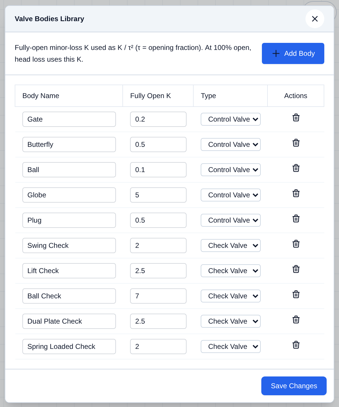
Open Data → Valve Bodies... to define fully-open minor-loss K values. Valves use K / τ², where τ is the opening fraction, so head loss at 100% open is this K.

1. Open Data and choose Valve Bodies....
2. Edit a body or click Add Body.
3. Click Save Changes. Then pick the body on the valve.

Cost Estimator

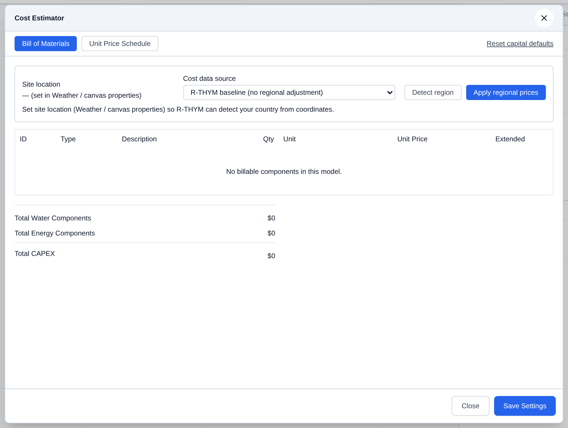
Open Data → Cost Estimator... for a project-level bill of materials (BOM) and the unit-price schedule behind it. Bill of Materials totals equipment from the canvas at those unit prices. Site Location can seed regional defaults. Other acronyms are listed in the Glossary.

1. Open Data and choose Cost Estimator....
2. Review the Bill of Materials.
3. Switch to Unit Price Schedule to edit the rates used in that total (tabs below).
4. Click Save Settings.

Unit Price Schedule

Click Unit Price Schedule. Five tabs set the rates behind the BOM and the operating cash-flow items: Capital, Development & Financing, Maintenance, Power, and Water Supply.

Capital

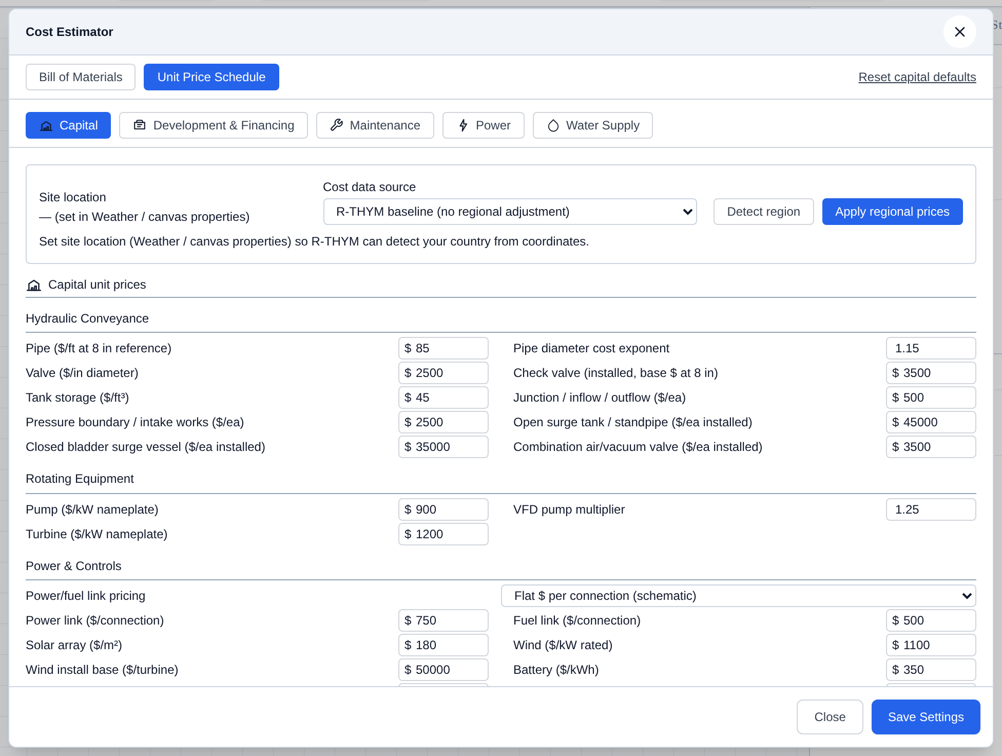
Capital is the unit-price book the BOM multiplies against canvas equipment. Groups include hydraulic conveyance (pipe, valves, tanks, surge devices), rotating equipment (pumps, VFDs, turbines), power and controls (links, solar, wind, batteries, interconnection), and fuel generators by type. Power/fuel links can be priced as a flat connection or by diagram route length.

Development & Financing

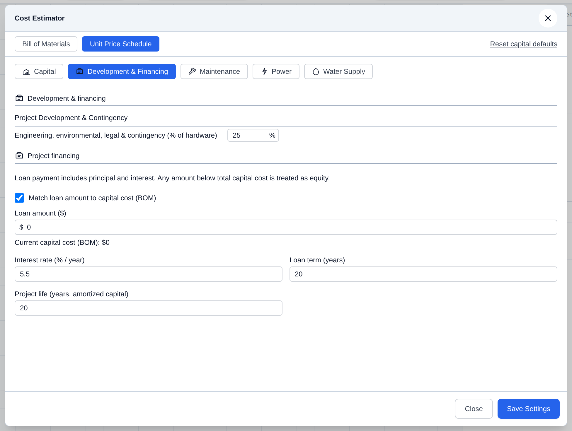
Development & Financing adds project overhead and the loan used to amortize capital. Engineering, environmental, legal & contingency is a percent of hardware (the BOM subtotal). Project financing sets loan amount (optional match to BOM capital), interest rate, loan term, and project life. Any capital not covered by the loan is treated as equity.

Maintenance

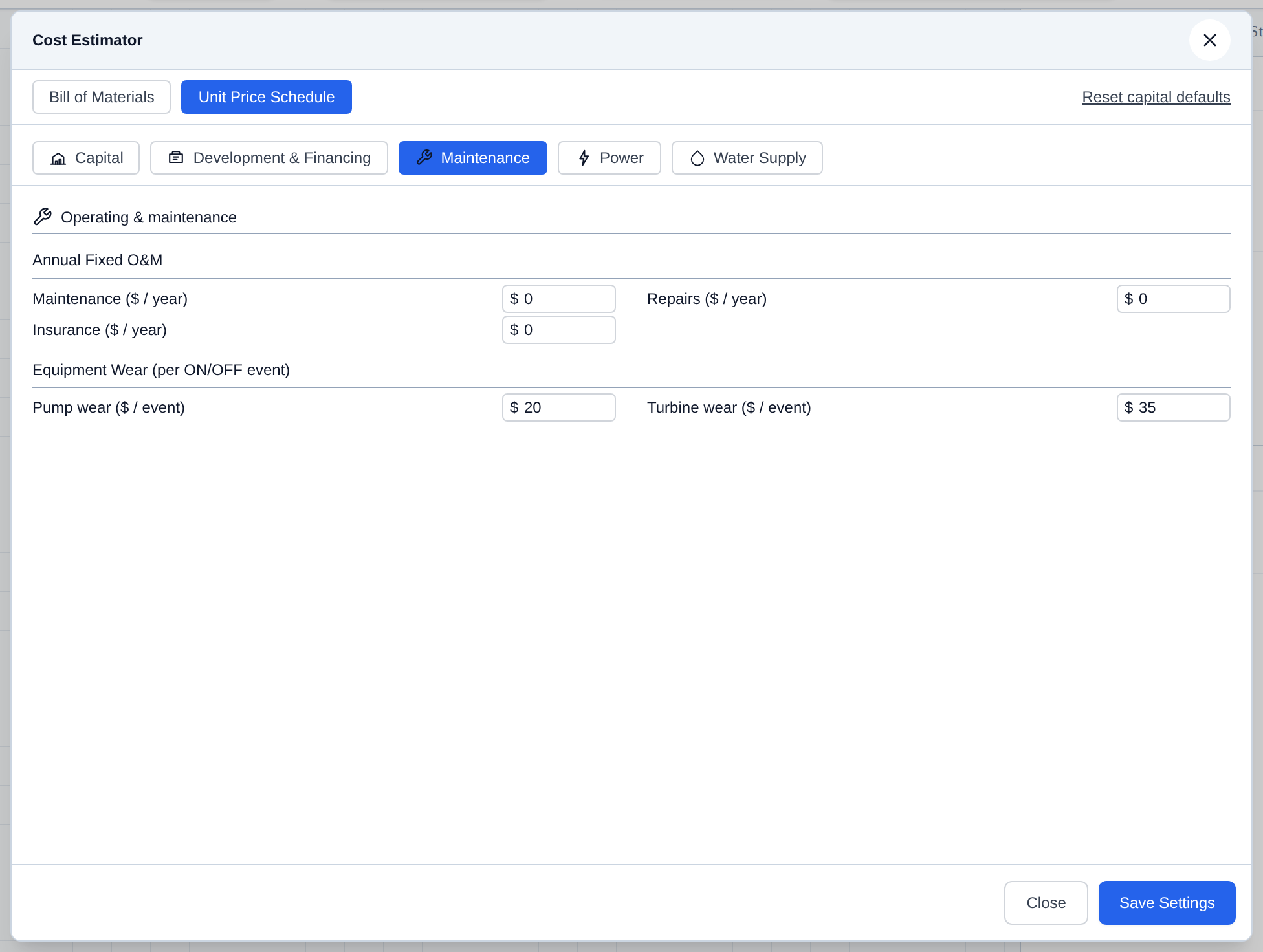
Maintenance is operating cost, not CapEx. Annual Fixed O&M is yearly maintenance, repairs, and insurance. Equipment Wear charges a dollar amount each time a pump or turbine cycles ON/OFF.

Power

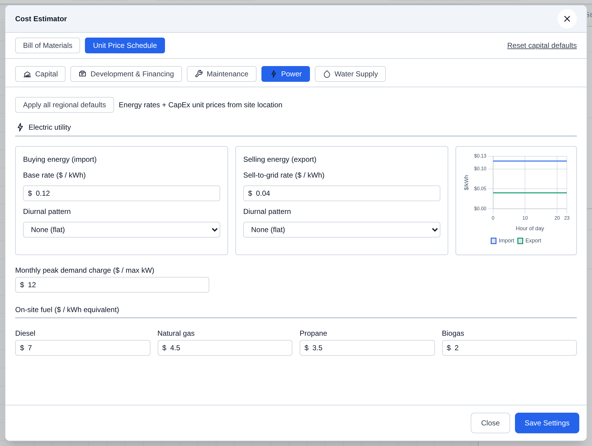
Power is the electric tariff and on-site fuel prices used in the energy cash flow. Set Buying energy (import \$/kWh and a diurnal pattern) and Selling energy (export \$/kWh and pattern), plus a monthly peak demand charge (\$/max kW). On-site fuel is \$/kWh equivalent for diesel, natural gas, propane, and biogas. Apply all regional defaults pulls energy rates and CapEx unit prices from Site Location.

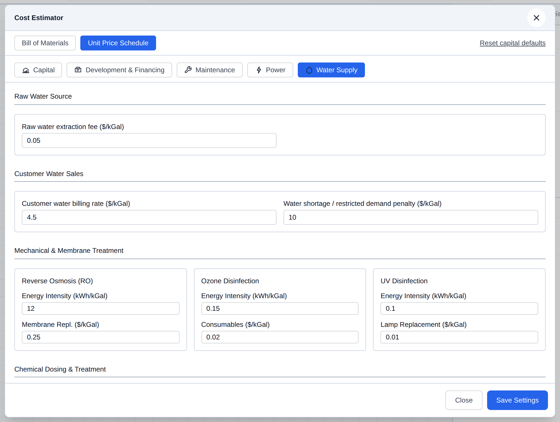
Water Supply

Water Supply prices water as a commodity and as treatment. Raw Water Source is the extraction fee. Customer Water Sales is the billing rate and a shortage/restricted-demand penalty. Mechanical & Membrane Treatment (RO, ozone, UV) has energy intensity and replacement/consumable costs. Chemical Dosing is bulk \$/kg for chlorine, coagulants, and pH adjustment. Volume units follow Edit → Units....